The The Forward Backward-Splitting Method (FBSM) Simply Explained
Using simple and understandable terms, along with code snippets (python) to provide a straightforward explanation

The FBSM isn’t just another tool in my Numerical Optimization Toolbox. Even though it tries to find the optimal value for an objective, accounting for additional function or constraints into account, just like other Methods.
Why is the FBSM important and what makes it so special?
Personally, the Algorithm played an important role to get in touch with the domain of Numerical Optimization. What made it so perfect is the simplicity of the underlying idea, which makes it easy to follow along while coding. Although it’s intuitive, it’s yet beautifully effective. But now let’s have a look at the idea
The Simple Idea Behind FBSM
In a nutshell the FBSM divides and conquers.
To give an abstract idea of the algorithm, it breaks down the optimization task into 2 manageable pieces, which are easier to work with. The algorithm iteratively switches between optimizing these 2 sub-tasks.
To put it into more concrete terms, FBSM splits the objective function h(x)into two pieces: f(x) and g(x), where:
- f(x) is a smooth function that is differentiable and represents a step in the direction we want to optimize
- g(x) is the non-smooth function that is a step in the direction of the constraints we want to take into account
In doing so, we are able to optimize the smooth and non-smooth parts of the objective function separately.
But now let‘s have a look into implementation.
I decided to go with an Object Oriented approach.
class FBSM:

    def __init__(self,
                 x,
                 parameters,
                 gradOpjective: function,
                 proximalOperator: function,
                 stepsize: float):

        self.gradObjective = gradOpjective  # gradient of the objective function
        self.proximalOperator = proximalOperator   # proximal operator for L1 regularization
        self.stepsize = stepsize   # size of steps
        self.x = x   # starting point
        self.params = parameters   # parameters for Objective


## Rest of the class ...
Class attribute descriptions:
- x — represents the vector starting point
- parameters — the parameters that need to be fed into the objective function h(x). In my case those are: M — matrix with double the width as height, y — vector with the same length as the height of M, tau — a positive scalar quantity
- gradObjective — gradient function of f(x)
- proximalOperator — the function g(x)
- stepsize — defines the length of the step taken in each iteration
Since we had a closer look at the class structure, let’s start with building the necessary methods for the forward step and backward step.
The Forward Step
## ...

   def forward (self):
        """
        The Forward Step moves in the direction of the negative gradient of the objective function
        """

        gradient = GradObjective(self.x, *self.params)
        x_k1 = self.x - self.stepsize * gradient
        return x_k1

## Rest of the class ...
During the Forward step we compute the gradient of the objective function h(x) with respect to the current position which is represented by the variable `x` and the parameters `params`.
The resulting vector we receive from this operation defines the direction in which we should go in order to minimize the problem (i.e. optimize it). Therefore we multiply this vector with our step-size and subtract the resulting value from our current position `x` to obtain our new position.
The Backward Step
## ...

    def backward (self, x_k1):
        """
        The Backward Step moves the new x into the direction of the Proximal Operator
        """
        return self.proximalOperator(x_k1)

## Rest of the class ...
For the Backward step we simply plug in the the current position into the proximal Operator. It’s idea is to find the closest point to the current position, in the set of the optimizers
Everything put together
    def solve (self, n_iterations = 1000, tol =1e-6):
        """
        Performs the Forward and Backward steps iteravely until the limit of iterations is reached or the distance moved falls below the tolerance.
        """
        steps = []

        for i in range(n_iterations):

            steps.append(self.x) #let's append the start as step or the last backward step
            x_k1 = self.forward()

            steps.append(x_k1) #let's append the last forward step
            x_k1 = self.backward(x_k1)

            distance = np.linalg.norm(self.x - x_k1) #compute the traveled distance during one forward and backward step

            if distance < tol:
                break

            self.x = x_k1

        return self.x, np.asarray(steps)
Now we have everything we need. Namely the Forward Step and the Backward Step.
Let’s put it all together and create a method which iteratevly performs a forward and a backward step until the distance traveled in an optimization step is smaller than a certain threshold (tolerance) `tol` or the number of steps exceeds the maximum steps `n_iterations`.
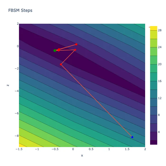
Additionally, because solely returning the final position is boring, we keep track of all performed steps and return them as well. This way we can see how the method performed on the problem space and can better analyze its behavior.
In conclusion
The FBSM is a great starting point to peer into the world of Numerical Optimization and learn how to implement mathematical algorithms.
Despite how powerful FBSM is, its applicability is limited to problems with a convex component in the objective function.
However, when applied to problems lacking a convex component, the FBSM may not converge, which means that it is not guaranteed to find an optimal solution.
I’ve uploaded my complete Implementation, together with an exemplary Objective and problems, to Github. Please feel free to have a look. https://github.com/j-tobias/Forward-Backward-Splitting